Combining LEFT, SEARCH and VLOOKUP

To complete this tutorial, you will need to download and UnZip the following file from GoogleDrive; it contains two versions of the workbook used in the tutorial: the start version and the completed version.

Download the tutorial workbook(s)

In the download tutorial folder, open "04 Manipulating Text"; and then open the Excel file: "01-Combining LEFT, SEARCH and VLOOKUP".

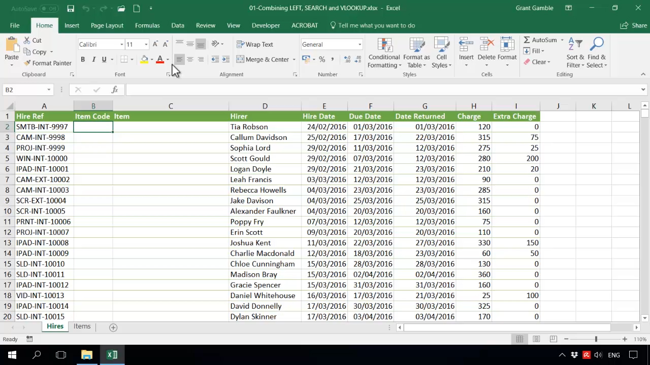
The workbook contains two worksheets. The first worksheet("Hires") has a record of the equipment hires that take place within an organisation. The code indicating which item was hired is embedded in the hire reference in column A.

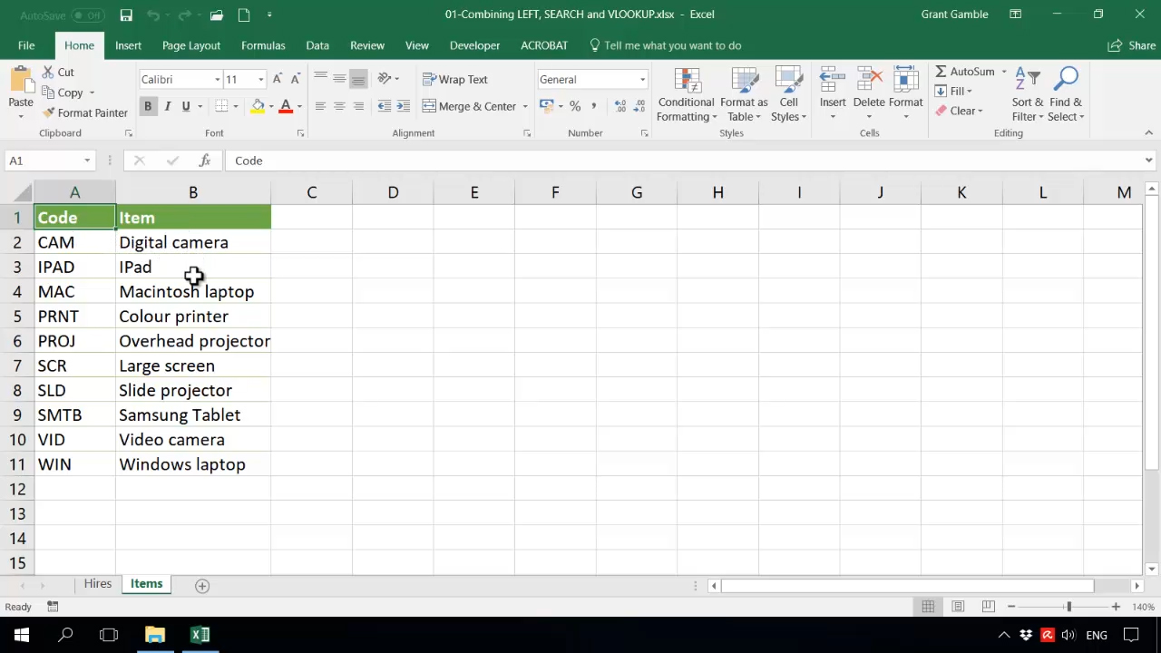
The second sheet ("Items") contains a lookup table detailing the piece of equipment indicated by each code.

Column A of the "Hires" table shows the Hire Ref(erence); but the Hire Ref has three components, separated by hyphens; and it is only the first of these components that matches column A of the "Items" worksheet. So, we need to come up with a formula which will extract all the text before the first hyphen.

On this occasion we cannot simply use the LEFT function on its own; because, when you use LEFT, you need to specify the number of characters to extract (starting from the left); and, in this example, the number of characters varies. Sometimes it is four, sometimes three.

Excel does, of course, have, in the Data Tab, a very useful feature called Text to Columns; but remember Text to Columns is an operation. What we are trying to do here is to create a formula which, given any hire reference, will extract the first component and then use the VLOOKUP function to find out the name of the corresponding item.

The name of the item is probably all we would need, in reality. However, just for practice, let us start by simply extracting the code; so that we can look at using two text functions in conjunction: LEFT and SEARCH.

Basically, what were interested in doing is extracting all of the characters which precede the first hyphen; so, we can begin by using the LEFT function.

The LEFT function takes two parameters: firstly, the text from which you want to extract a given number of characters; and this, of course, is the text in the cell A2.

The second argument is the number of characters to be extracted. However, in this example, we cannot simply provide a literal number. We cannot say three or four, because the number varies; so, instead, we use the SEARCH function to calculate this number, as shown in the diagram below.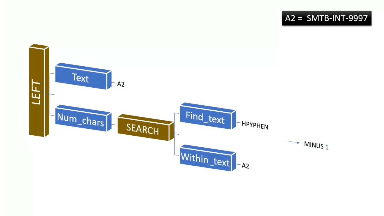

The SEARCH function becomes the second argument of the LEFT function: num_chars. The SEARCH function, in turn, takes two arguments. Firstly, we have the find_text; the text for which you are searching. And, secondly, the within_text; the cell in which you are looking for that text.

The SEARCH function returns a number, which is the character position of the string for which you are searching. In this case, in cell A2, the hyphen is in character position five, but of course we do not want to extract five characters. We always want to extract one character fewer than the character position of the hyphen. Therefore, after the closing parenthesis which ends the SEARCH function, we need to insert: "-1".

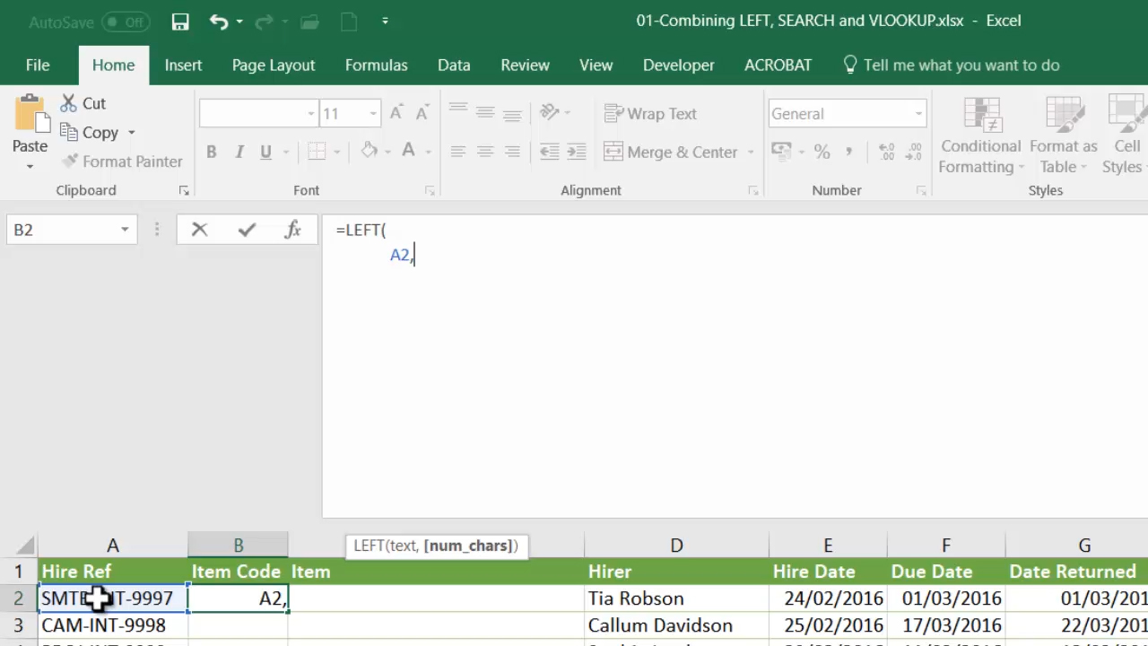
Let us enter our formula. Since we will be splitting the formula onto several lines, let us increase the size of the formula bar by clicking the expand button (the down-arrow on the right of the formula bar).

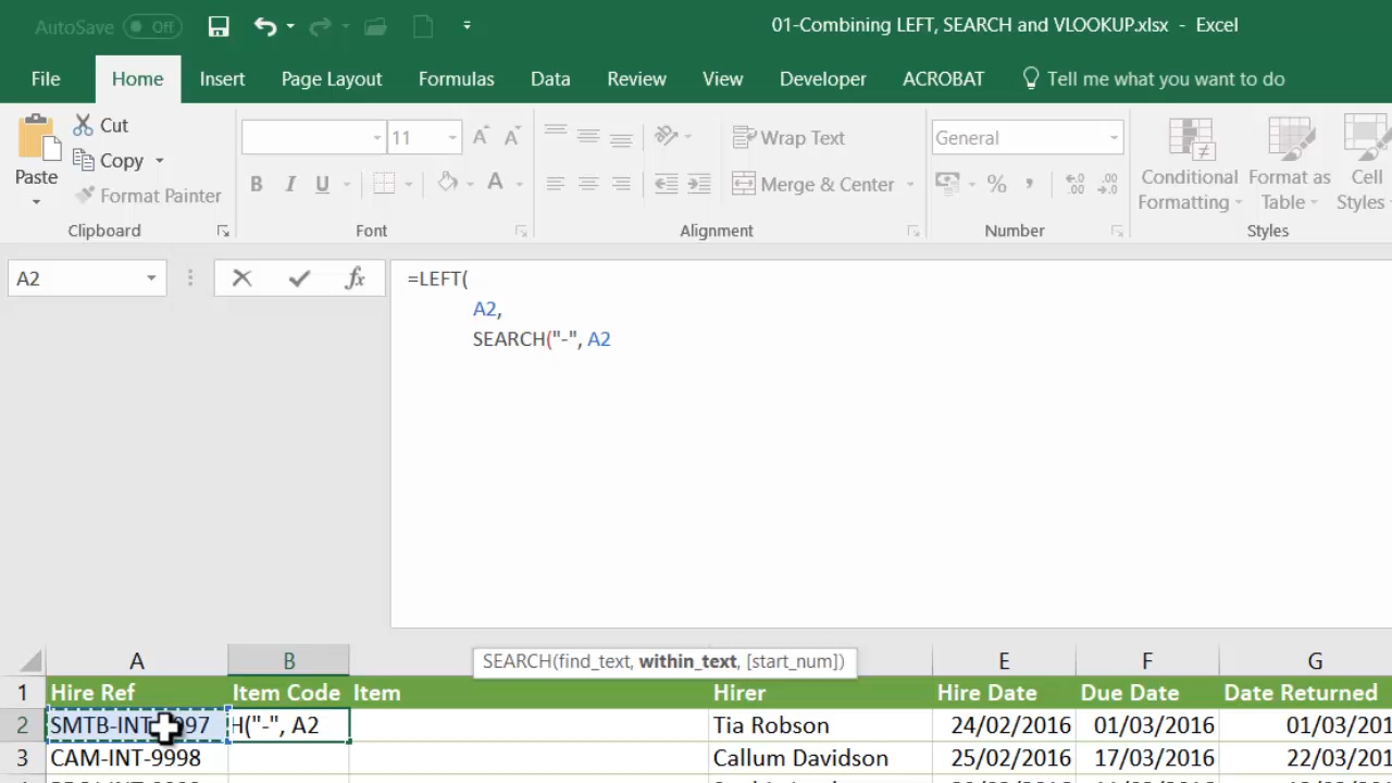
We begin by inserting: "=LEFT("; and then we press Alt-Enter to move to a new line within the formula bar and space to indent the next line under the opening parenthesis following the LEFT function.

Now, we insert the parameters (arguments) of the LEFT function. The first parameter is the text which, as you can see, is the text in the adjacent column A. Since our formula is in row 2 of the worksheet, we therefore click on A2 and Excel inserts the cell reference into our formula.

Your formula bar should now resemble the one shown in the illustration below.

Now, onto the second argument. Enter a comma, press Alt-Enter and then press the spacebar to indent the second argument of the LEFT function underneath the first.

For our second argument, we now need to use a function which will identify the character position of the first hyphen. Excel provides two candidates SEARCH and FIND; FIND is case sensitive, and SEARCH is not. For that reason, it is probably best to think of SEARCH as the standard function and then only use FIND on those occasions where you need to take the case into account.

Since the SEARCH function does not have any other functions nested inside it, we will now write the function and its arguments on a single line.

Enter the first argument of the SEARCH function (find_text) manually. Type: “SEARCH("-", ”; then, for the second argument, click on cell A2 to have Excel to insert the cell reference into the formula.

If we omit the third parameter (start_num), Excel will simply start searching from character one.

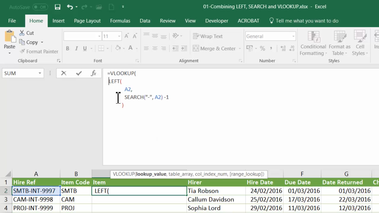
Once we have found the position of the hyphen, we need to subtract one. Thus, for example, in cell A2, the hyphen is in position five. Therefore, we do not want to extract the first five characters; we want to extract only the first four. So, we need to subtract one from the figure returned by the SEARCH function.

Thus the second argument of the LEFT function should read: “SEARCH("-", A2) - 1”.

To complete the formula, we press Enter and then use the space bar to position the cursor under the opening parenthesis which follows the LEFT function and we insert the closing parenthesis.

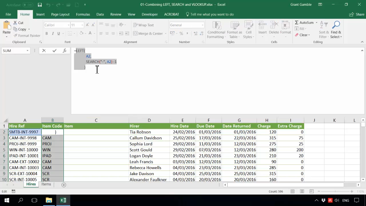
So, we now have a formula which extracts all the characters before the hyphen, rather than a fixed number of characters.

In reality, we probably would not bother to have a separate column just for the item code. All we really need to know is the name of the item which was hired; but, in a learning scenario, it is useful to have a look at these steps in isolation; to look at the components that go together to make up the whole.

Now, before entering the formula for the item column (in cell C2), in the formula bar, we can now highlight and copy the entire formula which we have just completed (apart from the equal sign); then press Escape to avoid accidentally modifying the formula. We can then paste this formula as the first argument of the VLOOKUP function which we will use in cell C2 to find the name of the item hired.

Next, in cell C2, we enter: “=VLOOKUP(“; then press Enter and use the spacebar to position the cursor just beyond the opening parenthesis which follows the VLOOKUP function; where we can now enter the first argument of the VLOOKUP function.

VLOOKUP requires four arguments. Firstly, we have the lookup_value; the item for which we are seeking a match.

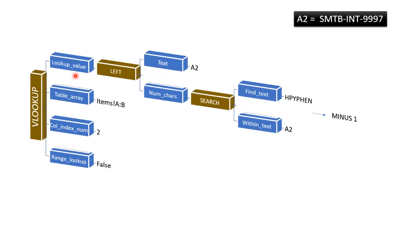
In this case, this is the code which will be extracted by our LEFT-SEARCH formula. So we simply paste in the formula we copied and use the spacebar to indent the arguments further in, to indicate that they now constitute the first argument of the VLOOKUP function.

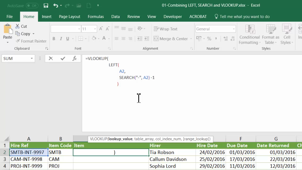
Next, we type a comma; Press Alt-Enter; and then use the spacebar to align the cursor under the first argument of VLOOKUP; namely, the LEFT function.

The second argument of the VLOOKUP function is the table_array, the columns in which we are looking for a value. We will be looking in the adjacent worksheet: “Items”. So, activate the “Items” worksheet and drag across column headings A and B, to create the cell reference: “Items!A:B”.

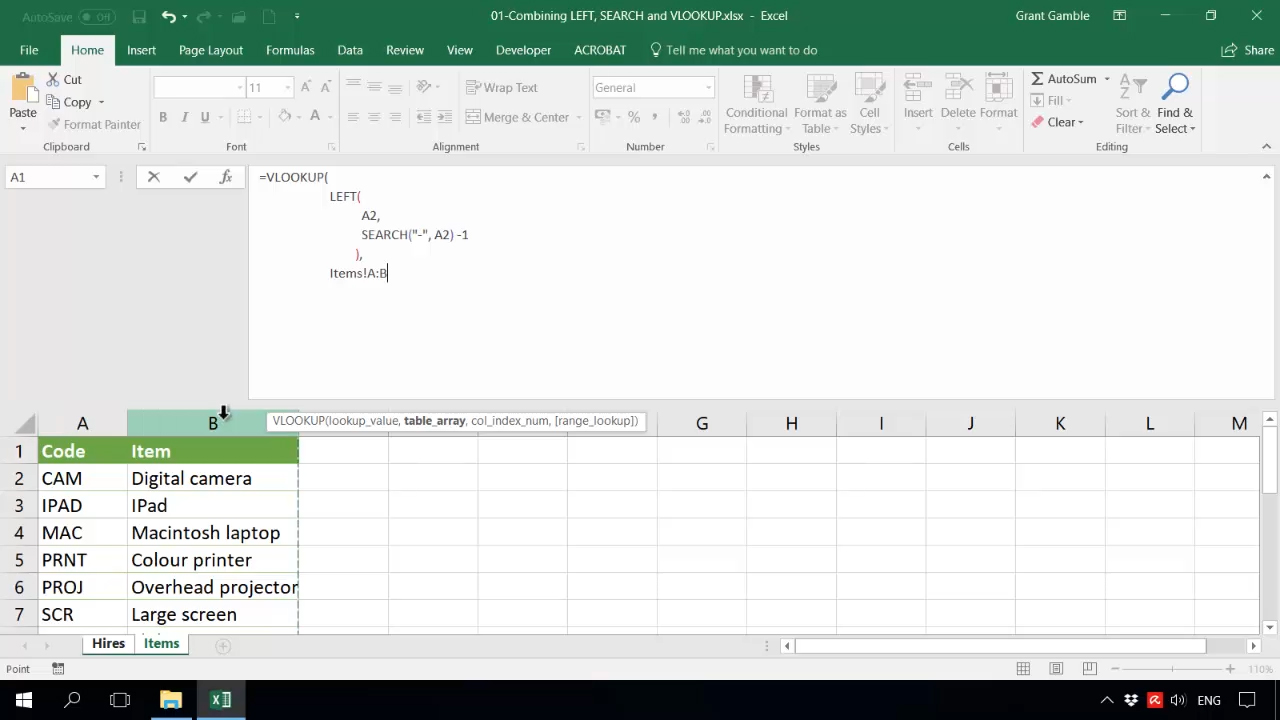
The third argument of VLOOKUP is the column_index number within the lookup table (which column contains the answer we are seeking); and it is always numeric.

So, we type a comma; Press Alt-Enter; and then use the spacebar to align the cursor under the first and second arguments of VLOOKUP. Then we simply enter the number two.

The fourth, and final, argument of VLOOKUP is the range_look_up, which specifies whether you are looking for an exact match or an approximate one. We are looking for an exact match. So, we type a comma; Press Alt-Enter; and then use the spacebar to align the cursor under the first, second and third arguments of VLOOKUP. Then we simply enter either FALSE or zero.

Finally, we press Alt-Enter; use the spacebar to align the cursor under the opening parenthesis which follows the VLOOKUP function and insert the closing parenthesis to complete the formula.

We can then copy this formula down into the cells below.

SUMMARY

In this tutorial, you have seen an example of how one (nested) function can serve as the argument of another (parent) function. In this example, the SEARCH function was nested as the second (num_chars) argument of the LEFT function; which, in turn, was nested as the first (lookup_value) argument of the VLOOKUP function.

Hopefully, you can also see the benefit of writing the formula on multiple lines; and of using the spacebar to indent the lines, to emphasize the hierarchical relationship between the various elements.