Nested IFs and Russian Dolls
When they hear the term “nested IFs”, a lot of people will visualize a structure whereby you have one parent IF statement with several IF statements nested inside it; and this is not actually the case.
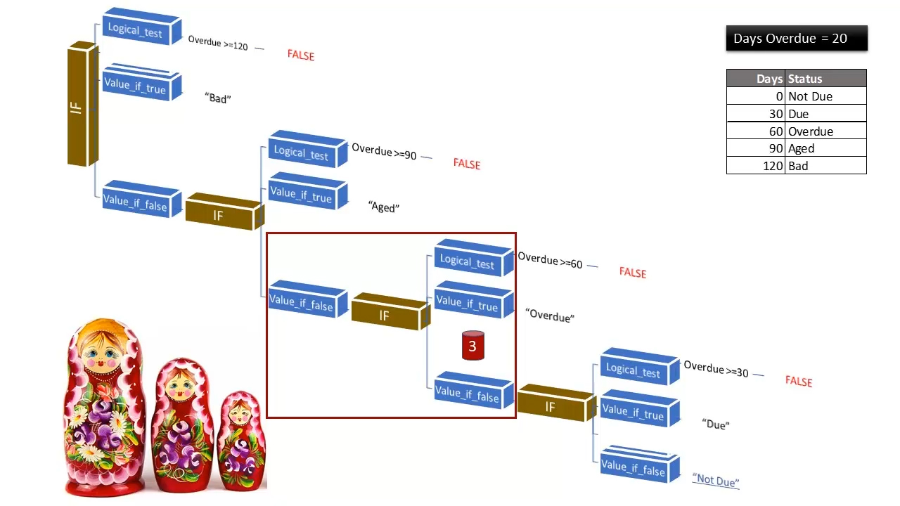
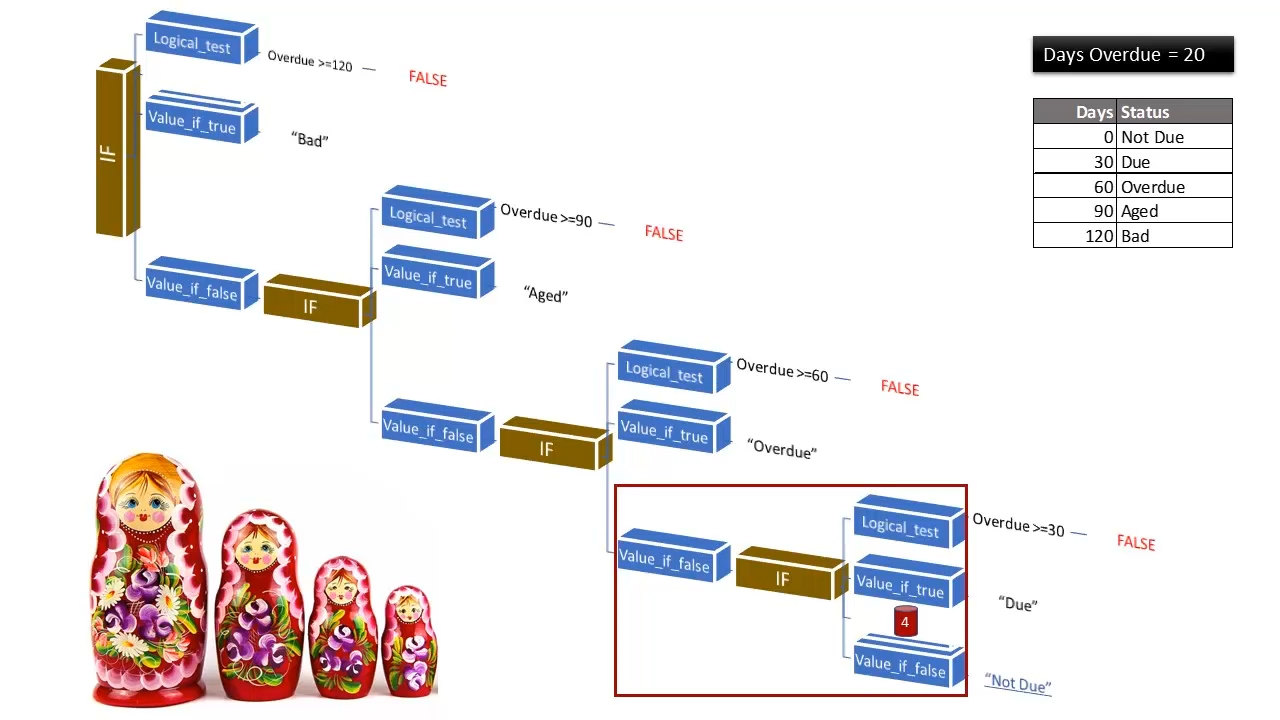
A better way of visualising nested IFs is to think of a Russian doll arrangement, whereby each IF statement is nested inside the previous one.
Click here to download the Excel workbook used in this tutorial.
Overview of our Nested IF Example
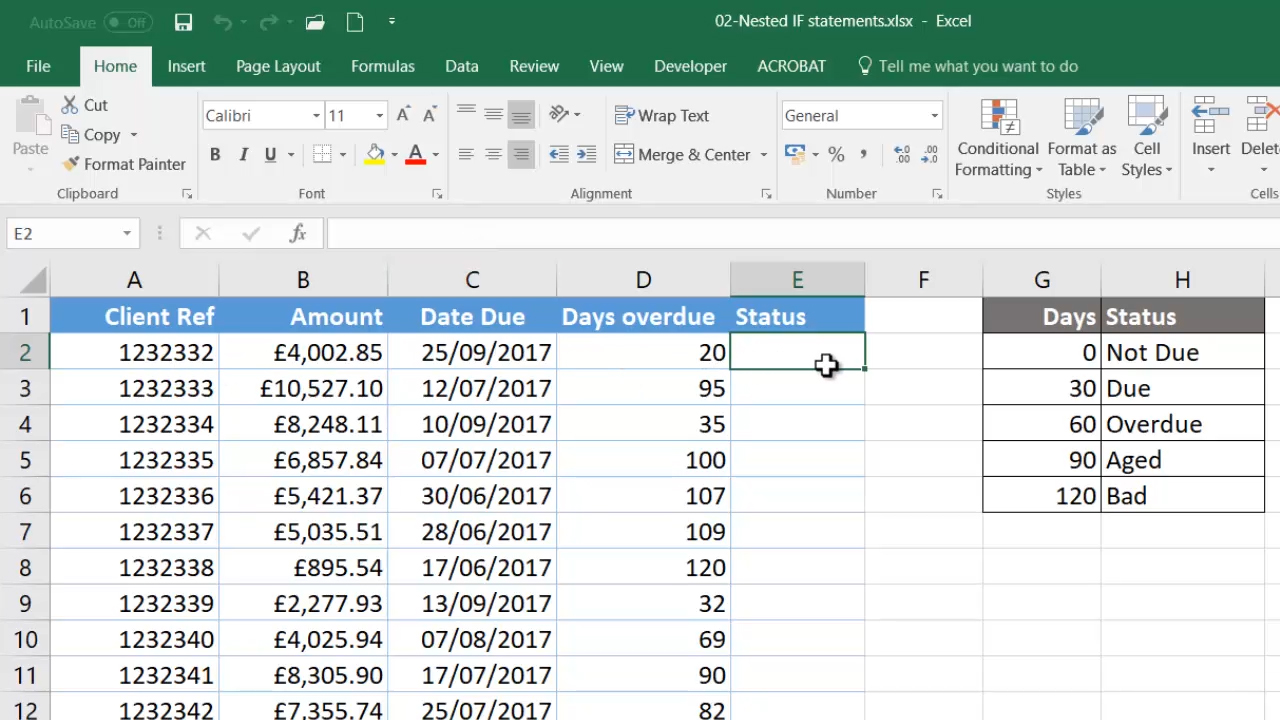
What we will be doing in this example is to assign a status to each of the accounts listed in this worksheet. The criteria that we will use to assign the account status are listed in cells G1 to H6.
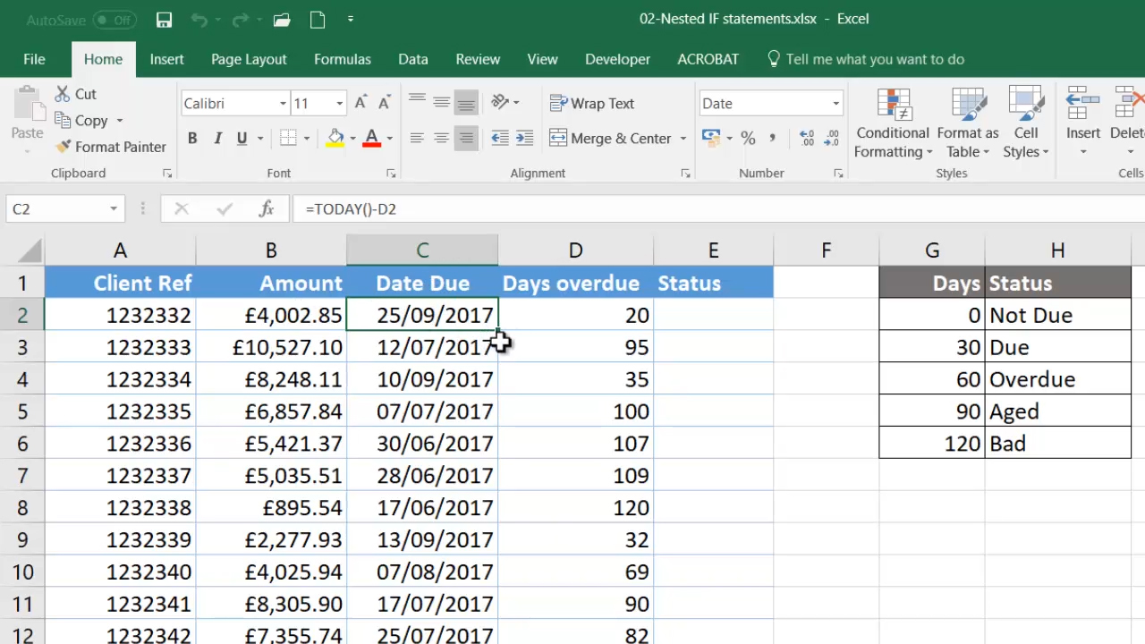
However, before we start discussing the formula, I should just explain one quirk that you will notice in this spreadsheet. The Days Overdue column contains static values and the Date Due column contains a calculation to display the date.
Obviously, in a real scenario, the reverse would be TRUE; we would have static values in the Date Due column and use a formula to calculate Days Overdue. This has been done for tutorial purposes; so that we can both have exactly the same data in column D.
To calculate the Status, we will use the criteria shown in columns G and H; thus, for example, 120 days overdue, or greater, indicates that the account status should be listed as “Bad”.
When you are using nested IF statements to test numerical values, it is always best to start with the highest value and work your way down to the lowest value. This means that you do not need compound testing; you do not need to say between 90 and 120, between 60 and 90, et cetera.
The reason for this is the way in which Excel evaluates the IF statements: it will stop evaluation as soon as it finds a TRUE value. Thus, by eliminating the highest value in our first test, when we perform our second test, we know that the value must be less than 120; because if it were not, the second test would never even take place. Hence, in each of our tests, we will simply use greater than or equal to; we will never need to use the less than operator.
How Nested IFs Work
Before we go ahead and write the formula, let us have a brief discussion of how nested IFs work.
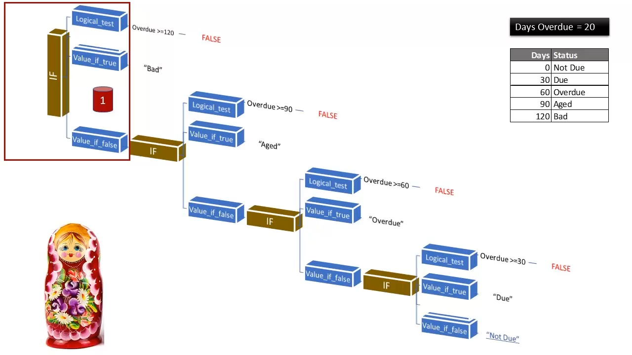
Staying with our days overdue example, let us say that we have a cell which contains 20 days overdue; and let us run this value through our nested IF structure. We start with our outer IF; the one that contains all the others. It has its usual three arguments: logical test, value-if-true and value-if-false.
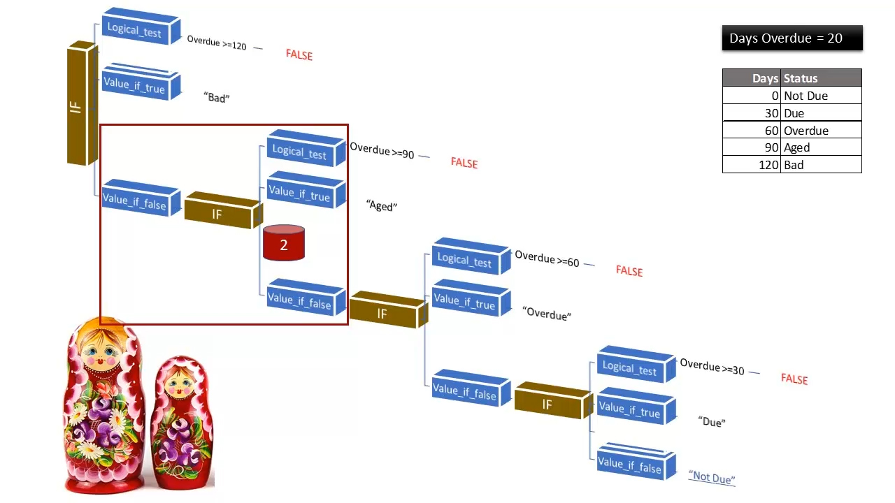
The logical test for the outer IF (days overdue greater than or equal to 120) proves to FALSE; but, instead of having a literal value as the result of this argument, we need to do some further testing. Thus, the value-if-false argument must be supplied by another IF statement; and this is how we end up with a second IF statement nested inside the first.
In the second IF statement, we are testing to see if the days overdue value is greater than or equal to 90; and, if it were, we would place the word “Aged” into the cell; but, since 20 is not greater than or equal to 90; we need the value FALSE. And, once again, since we have further testing to do, the value-if-false is supplied by another (the third) IF statement.
IF statement number three tests whether the value overdue is greater than or equal to 60. If it were, we would need the word "Overdue"; but since it is not, the value-if-false is the result; and this is supplied by the fourth and final, innermost, IF statement; in which we test whether the days overdue value is greater than or equal to 30.
The logical test argument of the fourth IF statement is the final test within the formula; and, once again, the test proves to be FALSE. However, now, since we have done all our testing, we can finally return the literal value: “Not due”.
So, as you can see, it is only the innermost IF that can ever have a literal value as the result of its value-if-false argument. The value-if-false argument of all the other IFs in the structure are, as it were, “hijacked” by nested IFs.
Writing the formula
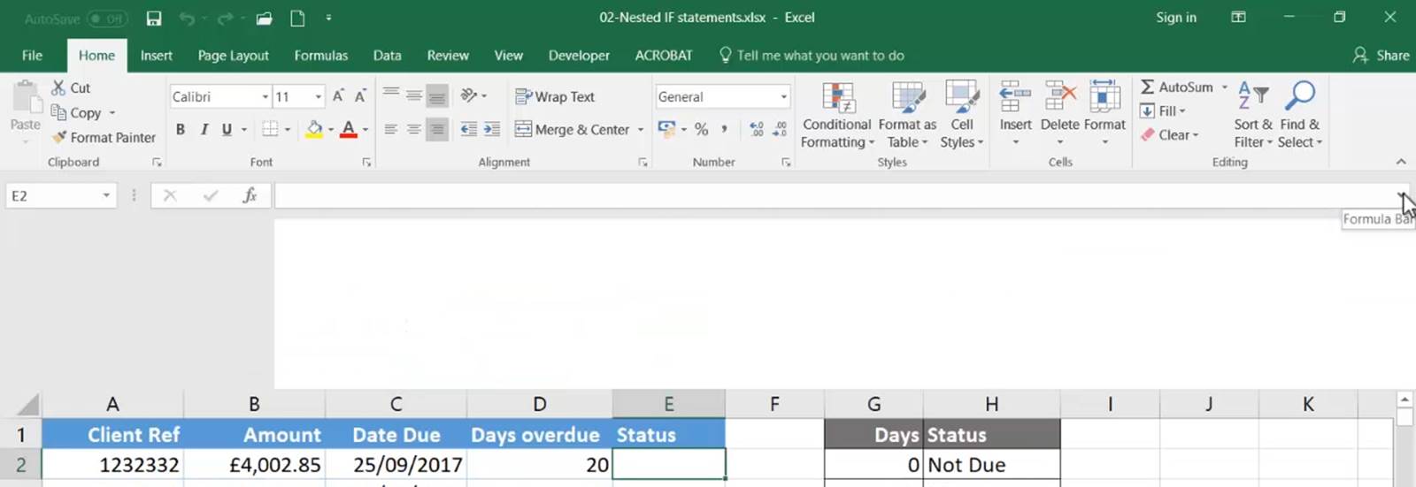
So, back to our workbook “Nested IF statements.xslx”, which you should have open on your screen (if you are following along with this tutorial). Let us increase the size of the Formula Bar, by clicking on the Expand/Collapse button, as shown below; so that we can split the formula onto multiple lines.
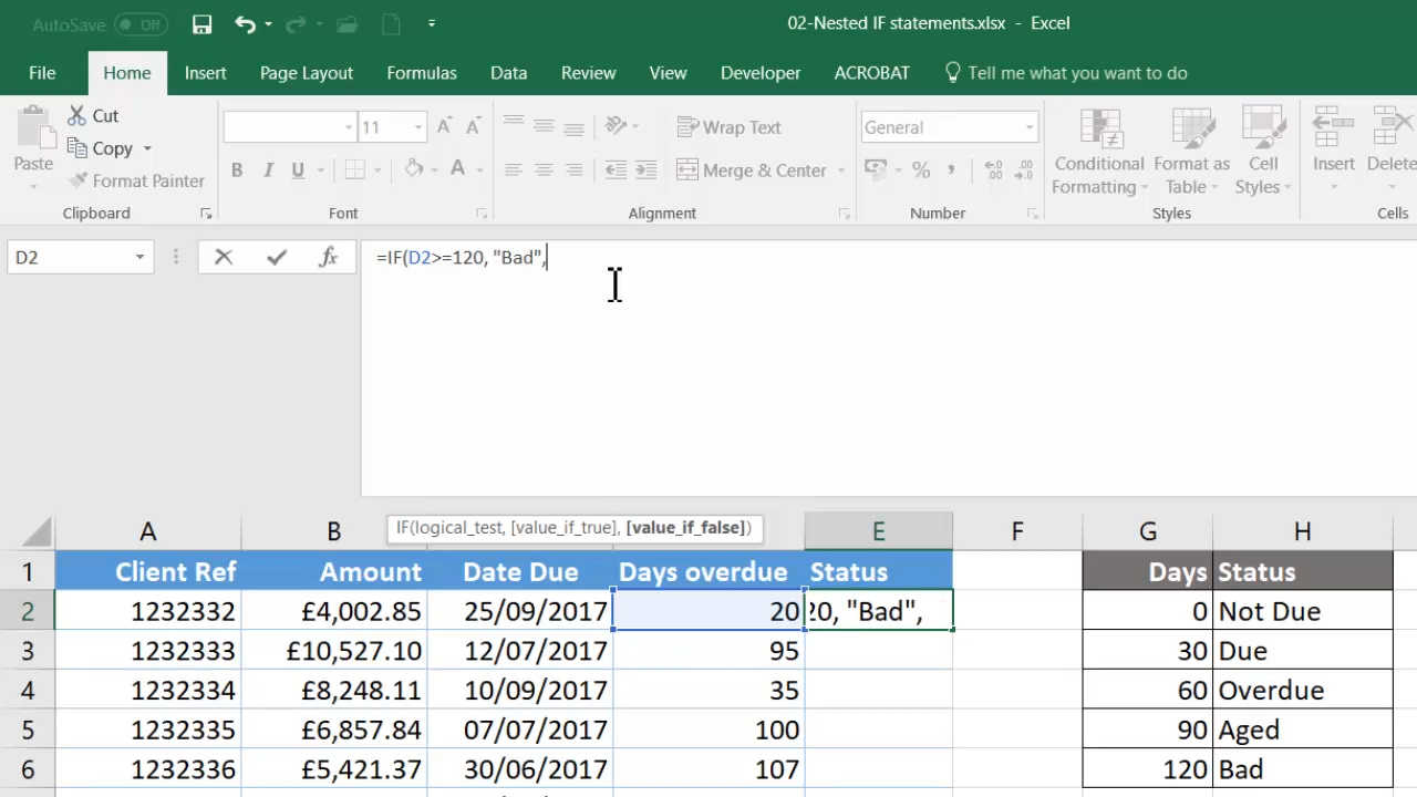
Click in the first data cell of the Status column: E2; and let us start with the first two arguments of the outer IF statement (logical test and value-if-true): =IF(D2>=120, "Bad", .
So, in plain English, what we have so far is: “If the value in cell D2 is greater than or equal to 120, then insert the word ‘Bad’ into cell E2”.
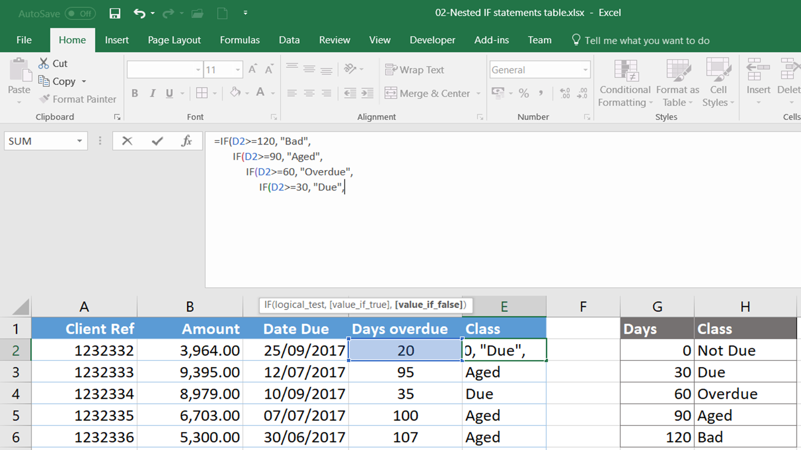
Since we need three further very similar tests, we can now highlight and copy the formula (minus the equal sign of course). Then, using Alt-Enter for a new line and the spacebar for indentation, we can paste the text that we have copied three times, each time indenting a little further to indicate the fact that each IF statement is supplying the third argument of its parent IF. (See below.)
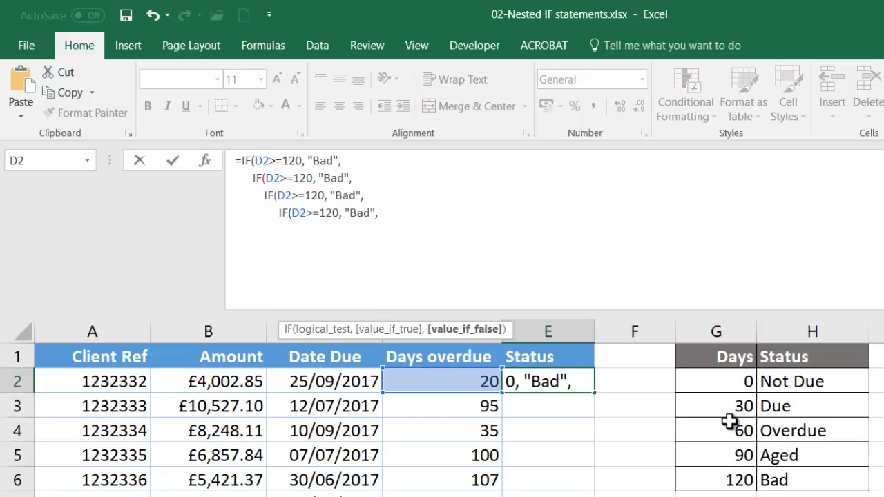
Then, all we need to do is to change the value-if-true argument to reflect the values shown in columns G and H of the worksheet. So, we end up with the values shown below.
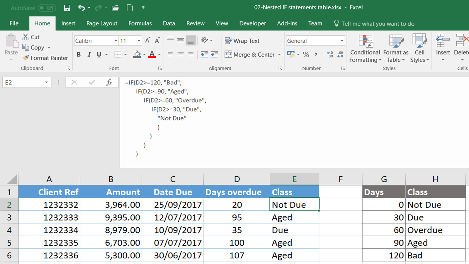
Having eliminated 120, 90, 60 and 30; we now know that, if none of these prove to be TRUE, the value-if-false needs to be the text “Not Due”.
So, we end the formula by inserting “Not Due” as the catch-all, value-if-false argument and by inserting a closing parenthesis to match each of four opening parentheses which followed our four IF statements (as shown below).
That completes our formula; so, we can restore the normal height of the Formula Bar and then copy the formula down.
That, then, is how nested IFs work; to understand them, just think of Russian dolls (unless you are one of those people who thinks that Russian dolls are much too full of themselves).
Nested IFs can become quite complex and convoluted; so, in the next two blog posts on logical functions, we will discuss two functions which provide an alternative to nested IF statements: IFS and VLOOKUP.

